KellyBoost:
A new way to construct portfolios
from machine learning models

Imagine a casino pays you even money on a coin that lands heads 60% of the time. You have a real advantage, so how much of your bankroll should you wager each round to maximize your profit?

In 1956, John Kelly at Bell Labs came up with the answer: 20%. Bet 20% of your bankroll, and your money will grow on average around 2% per round. Bet only 10%, and you keep only three-quarters of that growth, with less volatile swings. However, if you feel like pressing your advantage and bet an aggressive 40% every round, your long-run growth turns slightly negative. Same coin, same odds, but now you’ve slowly bet yourself to a loss.

In the world of sports betting and investing alike, the amount that you bet matters just as much as the prediction.

At the heart of this optimization question is the Kelly Criterion: a formula that calculates the size of your bet to maximize your long-run growth. It's powerful and unforgiving, because it penalizes you for playing your hand too big as well as for playing it too safe.

Maximizing this growth rate gives the optimal Kelly fraction f* = 2p − 1. With a 60% chance of winning, that means betting 20% of your bankroll.

Another layer of complexity in the world of unpredictable markets is that no one hands you the 60% edge; you have to find or create one using a model yourself.

Most machine-learning approaches to investing allocate their money in two steps. A predictive model forecasts what each asset will return, then an optimizer turns those forecasts into positions. The first step is prediction; the second is decision-making.

Another headache comes from the small bits of noise/errors that the optimizer amplifies.

A tiny forecast error becomes a big position, because the optimizer's whole job is to exploit even the smallest of differences between assets.

A forecasting model tries to minimize squared error, which means it is rewarded for being as correct as possible, while an asset allocation algorithm tries to find the best one relative to others given risk and return.

Put together, the two stages optimize for different goals, so improving the first doesn't necessarily lead to better results in the second.

A recent preprint by Jiayu Li tries to close that gap using a different portfolio management model, KellyBoost. It trains a gradient-boosted tree model directly on how fast a portfolio's wealth would have grown, so the model outputs portfolio weights and skips the forecast entirely.

Portfolio optimization had primarily used neural networks because backpropagation could help optimize different objectives, but boosted trees, the workhorse of tabular data, hadn't been explored as much because they needed custom gradient and curvature formulas for the loss.

The author derived both of these equations and tested their model against years of historical time-series data for a range of different assets.

So the question is: does this new approach work? Sort of, and that's the interesting part.

The direct approach using XGBoost beat a classification shortcut using LightGBM every time it was tested, but the old forecast-then-optimize pipeline still came out ahead.

But it's important to recognize the flaws in this model as well as possible changes and further experiments we could conduct to make it better.

For each decision date, the model produces one raw score per asset. A function called softmax converts those scores into portfolio weights: every weight is positive, and they add up to 100%.

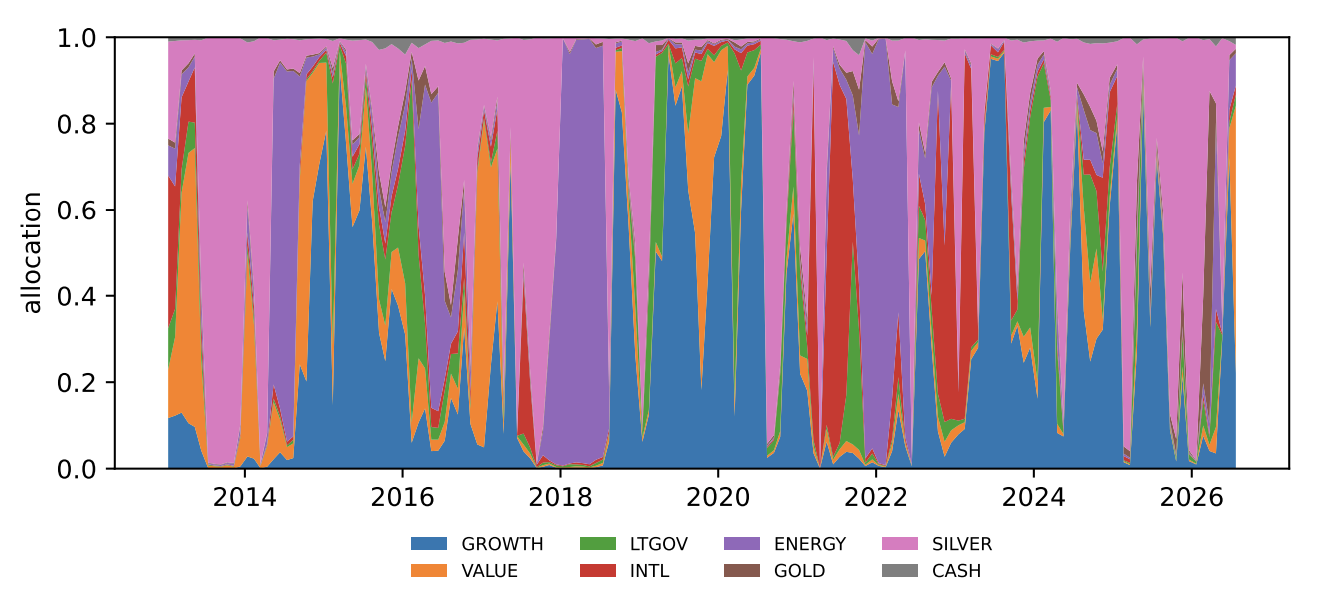
That means every decision is a full portfolio using the entire bankroll spread across many different assets. Every output of the model is the complete portfolio with no short positions and no optimizers in the middle.

Each period, the money is multiplied by (1 + your return). For a portfolio, that becomes:

Here, Wₜ is your wealth, wₜ is the vector of portfolio weights, and rₜ₊₁ contains the assets' returns in the following period.

By taking the logarithm, the chain of multiplications becomes a running sum, so the average log return becomes your long-run growth rate:

It's the same quantity that the Kelly bet in our coin example maximized. In this case, KellyBoost's "loss," the score it tries to make as small as possible, is just the negative of that growth. Minimize the loss over time, and you maximize growth.

This also takes away our need for a return forecast and a risk estimator.

The paper also proves what this loss is aiming at. A model with unlimited flexibility would learn, for every market situation, the best Kelly portfolio for that situation.

The loss is an average across situations, and the model can pick a different answer for each one, so each can be optimized on its own. In practice, the model is limited by noisy data, which is why the results section matters.

It can be easy to overlook the power of a boosted tree if you aren’t really familiar with how it works. Boosted trees learn by rounds. Each round adds a small decision tree that corrects what the previous rounds got wrong.

To do that, the algorithm needs two pieces of information for every asset on every date:

Here, S = wᵀy is the portfolio's realized return. If asset k beats the portfolio as a whole, then yₖ > S, making the gradient negative and pushing the model's score for that asset upward. The factor σₖ means the current portfolio weight matters, while1/(1 + S) captures the compounding effect of log growth.

Unlike a simple bowl-shaped loss, this objective is not convex in the raw scores, so hₖ can be negative. XGBoost needs positive curvature for its second-order update, so the implementation uses |hₖ|.

The fix is to use the curvature's absolute value. The paper shows this is safe: every update still moves downhill, and the fix only changes how big the steps are. It's the same trick as a known method called saddle-free Newton.

Neural networks get both automatically through backpropagation, a process by which it sends its output back in the other direction, working through and optimizing their weights to get the best possible outcome.

Boosted trees have no such routine, so someone has to hand them the formulas. Writing those out for the Kelly loss is the paper's core contribution.

The author checked them numerically, nudging the inputs slightly and confirming the formulas match the actual change in the loss. The derivations can be found in the appendix of the paper.

Why the model is trained four times

Boosted trees can be chaotic. Delete a single row from the training data, about 0.02% of it, and the model's final weights can shift by several percentage points because two nearly tied choices can flip.

So the paper trains four versions, each missing a different row, and averages their weights. This makes the output stable and reproducible without changing what the tuned settings mean.

As we'll see, it doesn't add any growth.

Li tested KellyBoost on eight assets: growth stocks, value stocks, long Treasuries, international stocks, energy, gold, silver, and cash.

The data runs from 2003 to 2026 and was split like a practice exam and a real exam:

That gives a small sample of 163 monthly decisions, which matters for everything below.

Two important terms: the Sharpe ratio is return per unit of risk, while maximum drawdown is the worst peak-to-trough drop in the portfolio's value.

Supporting Figures

KellyBoost results

Supporting figures from the KellyBoost analysis.

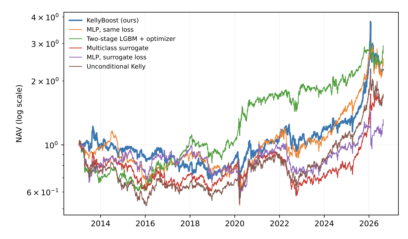
KellyBoost finished third out of six models, ahead of the fixed portfolio and both of the shortcuts.

Beating the fixed portfolio suggests the signals carry some information, though the margin is small. However, the author is upfront that with only 163 decisions, none of these gaps are convincing enough to be considered a real edge.

Test 1: Does training on growth beat a shortcut?

To isolate the effect of the training goal, the author trained both tree models and neural nets two ways: directly on portfolio growth, or on a classification shortcut, where the model learns to guess which asset will win the month and uses its confidence as the portfolio.

The shortcut discards information, because a month won by 0.2% counts the same as one won by 20%. Growth training won in all four matchups:

The direction was consistent, but the size, about +0.18 per month pooled, isn't statistically conclusive.

Test 2: Does a better optimizer help?

Next, the author swapped the exact curvature from the derivation for cruder substitutes and compared the practice-exam score to the real-exam score.

The more faithfully the model optimized, the worse it did when deployed. The crude version took timid steps, so its portfolio stayed closer to equal weights.

Its Sharpe ratio was double, and its worst drawdown was about half as deep.

The paper's explanation is that the exact version does precisely what it was asked: it estimates the growth-optimal portfolio, which is aggressive.

It banked its biggest year in 2025, but paid for the aggression in 2014–2018 and again in 2026, when its estimated edge turned out to be too optimistic.

The two-stage approach wins for a similar reason: monthly returns are barely predictable, so its forecasts sit near zero and its optimizer holds a mild, diversified portfolio.

Test 3: What did the signal search buy?

The author also let each method search 7,871 candidate signals for the ones that worked best in development.

Searching roughly doubled every method's practice score, but real-exam results diverged: the two-stage approach doubled (0.38 to 0.82), KellyBoost edged up (0.39 to 0.47), and both neural nets got worse (0.67 to 0.56, and 0.49 to 0.20).

When a method improves far more in practice than in the real test, it has likely been fitting noise, which the paper calls "selection bias made visible."

KellyBoost's final list is just five signals: statistical summaries of international equity, wheat, copper, and soybean movements, plus financial-sector skewness.

The paper says it leaves the economic sense of that list "to the reader," and a fair reader will wonder why crop prices should drive a stock-and-bond allocation.

The paper fills a real gap. Up until now, decision-focused learning, one of the best ideas in applied ML where you train a model on the outcome you care about instead of a derivative, was only done through neural networks.

The KellyBoost model showed that a more favorable model for tabular data, boosted trees, could be applied the same way.

The model that followed the math most precisely optimized best in practice runs but worse once deployed — while a cruder, more cautious version came out on top.

Kelly is the best example, because it sizes bets directly from the estimated edge, and estimated edges in markets are mostly error.

Here's how expensive that error is, going back to our coin example. Suppose the true chance of heads is 55%, but your model says 60%. The right bet is 10%, which grows your bankroll about 0.5% per round.

Your model tells you to bet 20%. At a true 55% edge, that bet grows your bankroll by roughly nothing.

Five points of overconfidence erased the entire edge. That asymmetry is why practitioners use fractional Kelly, and why the paper's "constant curvature" variant, accidentally cautious, had half the drawdown and double the Sharpe.

Why we'd be cautious about the paper itself

None of this is a knock on the author, who flags most of it. It's a checklist for reading any academic paper, including this one:

• Small sample. 163 monthly decisions. Every pairwise gap in the main table has a confidence interval that includes zero, including the 4-of-4 result the paper's claim rests on (pooled interval −0.11 to +0.50).
• Search creates its own luck. The model picked five features out of 7,871 candidates, and development scores roughly doubled while deployed scores didn't follow.
• Feature selection is economically unclear. The final list includes wheat, copper, and soybean quantiles driving a stock, bond, and metals allocation, which is a classic warning sign for data mining.
• The first pipeline underperformed. The feature search was added in response to that performance, and the paper says so openly.
• One preprint, one universe, no peer review. Eight assets, long-only, main results before costs, and a single author.

This is more of an experiment than a fully explored strategy, but it’s important to notice the potential it could have.

Replicating this to shorter timeframes or including other assets could possibly turn this into a valid strategy, but it would require more robust dataset selection and training.

What to take from it

1. Ask what your model is being rewarded for, and whether that's the outcome you care about.
2. Ask what happens to the strategy when the inputs are wrong, since they will be.
3. Distrust any result that improves more in development than in deployment.